
2016년 3월에 있었던 알파고(AlphaGo)와 이세돌의 딥마인드 챌린지 매치 이후 딥러닝의 열기가 가시지 않고 있는데요. 그 중요성은 점점 더 커지고 있으며, 바이오 분야에서도 그 바람이 불고 있는 것 같습니다.
딥러닝이란 Layer를 쌓아서 학습시키는 기계학습 방식을 지칭합니다. 입력층, 은닉층, 출력층 등 단 3개의 층만으로 모든 형태의 함수를 구현할 수 있다는 게 수학적으로 증명되었고, 이를 보편근사이론(Universal Approximation Theorem)이라고 합니다. 하지만 3개의 층으로만 구성하게 되면 학습에 오랜 시간이 걸리기 때문에 여러 개의 층을 생성하여 딥러닝을 구현하는 게 일반적입니다. 이를 이미지에 응용한다면 이미지의 픽셀을 일렬로 줄을 세운 뒤 은닉층의 노드들과 Fully Connected Network(FCN)를 만드는 것을 생각할 수도 있을 것입니다. 하지만 이러한 Fully Connected Layer(FCL)는 파라미터가 굉장히 많이 필요하기 때문에 메모리 소모가 크고 학습 시간이 오래 걸려 현실적이지 않다는 비판을 받아왔습니다.
이러한 배경 하에 합성곱 신경망(Convolutional Neural Network, CNN)이 대두되었습니다. 이 신경망은, 공간상에서 가깝게 위치한 벡터끼리 내적을 하면 큰 값이 나온다는 것에서 착안하여 이미지 국소 부위의 특정 패턴을 인식하기 위해 벡터의 내적을 활용합니다. 이때 이미지 국소 부위는 이미지 일부분의 픽셀들을 일렬로 줄을 세운 하나의 벡터로 표현할 수 있을 텐데, 이와 대응되는 또다른 벡터를 필터(Filter)라고 합니다. 이러한 접근 방법을 취하는 데 있어서 크게 두 가지 가정이 필요합니다.
- Spatial Locality : 이미지 일부분으로부터 얻은 패턴들을 재구성하면 빠짐없어 전체 패턴을 구해낼 수 있다는 것
- Positional Invariance : 위치, 시선각에 상관 없이 동일한 패턴을 인식할 수 있다는 것
합성곱 신경망은 매 Layer마다 학습해야 하는 파라미터는 FCN이 아니라 필터이므로 Computing Burden을 줄일 수 있습니다. 또한, 이미지 부분별로 얻어지는 연산값을 모으면 하나의 이미지가 될 수 있기 때문에 Layer마다 새로운 이미지가 생성됩니다.
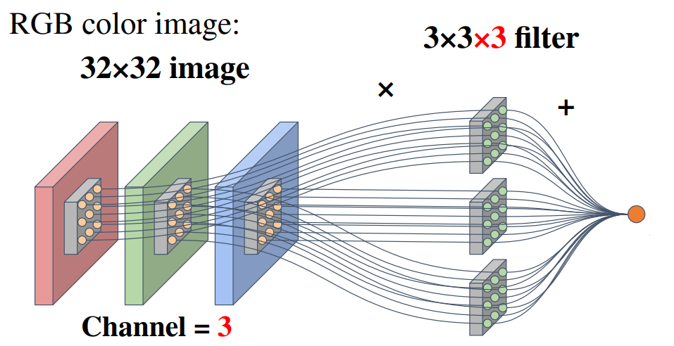
위 예시에서는 32 × 32 × 3 (= W × H × C)이 입력으로 주어져 있고, 3 × 3 × 3 필터를 이용하고 있습니다. 채널(Channel, C)에는 대표적으로 RGB 채널이 있으며, 필터는 일반적으로 3 × 3을 사용합니다. 위 그림은 Element-wise하게 곱하여 전부 더하는 식으로 내적을 구현하고 있음을 알 수 있고, 일반적으로 바이어스 항을 더해주는 데 그 항이 생략돼 있다는 것을 주의해야 합니다. 위와 같이 3 × 3 × 3 필터를 한 칸씩(S = 1) 가로, 세로로 이동시키면 은닉층에서 변형된 이미지는 30 × 30 × 1이 될 것입니다. 3 × 3 × 3 필터가 K개가 있다면 은닉층에서 변형된 이미지는 30 × 30 × K (= W' × H' × K)가 될 것입니다. 이를 요약하면 다음과 같습니다.
- W : Width
- H : Height
- C : 입력층의 채널 수
- K : 출력층의 채널 수
- F : 필터의 크기(Filter size, Kernel size) (단, 위 예시의 경우 3)
- S : Stride
- P : Zero padding
- W' = (W - F + 2P)/S + 1
- H' = (H - F + 2P)/S + 1
- CNN의 파라미터의 수 = K(F2C + 1) (단, 1은 바이어스를 의미)
- FCN의 파라미터의 수 = (W × H × C + 1) × (W' × H' × K) ≫ K(F2C + 1)
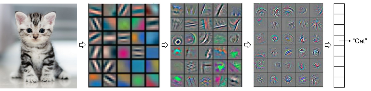
실제로 이와 같이 구성을 하면 각 Layer는 특정 패턴을 인식하게 됩니다.
이러한 CNN 알고리즘의 퍼포먼스를 높이기 위해 Augmentation Layer, Pooling Layer, BatchNormalization, Flatten, Dense, Dropout 등이 같이 사용되고 있습니다. 다음은 자주 사용되고 있는 TensorFlow의 API입니다.
tf.keras.layers.Conv2D(
    filters,
    kernel_size,
    strides=(1,1),
    padding="valid",
    data_format=None,
    dilation_rate=(1,1),
    groups=1,
    activation=None,
    use_bias=True,
    kernel_initializer="glorot_uniform",
    bias_initializer="zeros",
    kernel_regularizer=None,
    bias_regularizer=None,
    activity_regularizer=None,
    kernel_constraint=None,
    bias_constraint=None,
    **kwargs
)
이제 이를 응용한 SPADE 알고리즘에 대해 알아보도록 하겠습니다.
- 풀 네임 : Spatial Gene Expression Patterns by Deep Learning of Tissue Images
- 출처 : Bae, S., Choi, H., & Lee, D. S. (2021). Discovery of molecular features underlying the morphological landscape by integrating spatial transcriptomic data with deep features of tissue images. Nucleic acids research, 49(10), e55-e55.
SPADE 알고리즘은 공간전사체(Spatial Transcriptomics, ST)를 다채널 이미지로 재해석하여 다른 광학적 이미지와의 결합을 시도하고자 한 최초의 시도로 크게 다음과 같은 파이프라인을 가지고 있습니다.
- 각 ST 스팟에 대응되는 H&E 이미지 조각을 얻습니다.
- 그 조각을 Pre-trained CNN (VGG16)에 입력으로 넣습니다.
- 최종적으로 512차원의 Feature를 얻습니다. CNN 알고리즘은 매 Layer마다 변형된 이미지를 얻으므로 이것이 가능한 것이죠. 한편, Feature를 패턴이라고도 합니다.
- 512차원의 Feature를 PCA로 차원을 축소합니다. 이러한 차원축소는 패턴을 재조합하여 Reconstructed Image를 얻는 것과 유사하다고 할 수 있습니다.
- 이때 얻어진 PC1, PC2, ... 등등은 제각기 다른 Physiological Meaning을 가질 수 있습니다.
다음은 실제 SPADE 알고리즘의 코드입니다.
### Python Code ###
import os
import numpy as np
import matplotlib.pyplot as plt
from skimage import draw
import pandas as pd
import argparse
os.environ['KERAS_BACKEND'] = 'tensorflow'
from keras import backend as K
K.set_image_data_format='channels_last'
from keras.applications import vgg16
from keras import backend as K
from sklearn.manifold import TSNE
from sklearn.decomposition import PCA

#Image Show
def spatial_featuremap(t_features, img, pd_coord_tissue, imscale, radius = 10, posonly=True):
    tsimg = np.zeros(img.shape[:2])
    tsimg_row = np.array(round(pd_coord_tissue.loc[:,'imgrow']*imscale), dtype=int)
    tsimg_col = np.array(round(pd_coord_tissue.loc[:,'imgcol']*imscale), dtype=int)
    for rr, cc,t in zip(tsimg_row, tsimg_col,t_features):
        r, c = draw.circle(rr, cc, radius = 10)
        if posonly:
            if t>0:
                tsimg[r,c]= t
        else:
            tsimg[r,c]=t
    return tsimg

if __name__ == "__main__":
    parser = argparse.ArgumentParser()
    parser.add_argument('--patchsize', type=int, default=32)
    parser.add_argument('--position', type=str)
    parser.add_argument('--image', type=str)
    parser.add_argument('--scale', type=float)
    parser.add_argument('--meta', type=str)
    parser.add_argument('--outdir', type=str, default='./SPADE_output/')
    parser.add_argument('--numpcs', type=int, default= 2)
    args = parser.parse_args()

    if not os.path.exists(args.outdir):
        os.makedirs(args.outdir)

    #Param
    sz_patch = args.patchsize

    br_coord = pd.read_csv(args.position,
                           header=None, names= ['barcodes','tissue','row','col','imgrow','imgcol'])
    br_meta = pd.read_csv(args.meta)
    if 'seurat_clusters' not in br_meta.columns:
        print("Warning: meta data including seruat_clusters show t-SNE map of image features with clustering info")
    else:
        print('Meta data is loaded')
    br_meta_coord = pd.merge(br_meta, br_coord, how = 'inner', right_on ='barcodes' , left_on='Unnamed: 0')

    brimg = plt.imread(args.image)
    print('Input image dimension:', brimg.shape)

    brscale = args.scale
    br_coord_tissue = br_meta_coord.loc[br_meta_coord.tissue==1,:]

    #Image Patch
    tsimg_row = np.array(round(br_coord_tissue.loc[:,'imgrow']*brscale), dtype=int)
    tsimg_col = np.array(round(br_coord_tissue.loc[:,'imgcol']*brscale), dtype=int)

    tspatches = []
    sz = int(sz_patch/2)
    for rr, cc in zip(tsimg_row, tsimg_col):
        tspatches.append(brimg[rr-sz:rr+sz, cc-sz:cc+sz])
    tspatches = np.asarray(tspatches)
    print('Image to Patches done', '....patchsize is ', sz_patch, ' .... number of patches ' , tspatches.shape[0])

    #pretrained model
    pretrained_model = vgg16.VGG16(weights='imagenet', include_top = False, pooling='avg', input_shape = (32,32,3))
    X_in = tspatches.copy()
    X_in = vgg16.preprocess_input(X_in)
    pretrained_model.trainable = False
    print('Architecture of CNN model')
    pretrained_model.summary()

    if 'seurat_clusters' in br_meta.columns:
        Y = np.asarray(br_meta['seurat_clusters'])

    #feature extraction
    ts_features = pretrained_model.predict(X_in)
    print('Image features extracted.')
    ts_tsne = TSNE(n_components=2, init='pca',perplexity=30,random_state=10).fit_transform(ts_features)
    print('t-SNE for image features ... done')

    plt.figure(figsize=(8, 7))
    if 'seurat_clusters' in br_meta.columns:
        plt.scatter(ts_tsne[:, 0], ts_tsne[:, 1], c=Y, cmap='Dark2' , s = 5, alpha=0.5)
    else:
        plt.scatter(ts_tsne[:, 0], ts_tsne[:, 1], s = 5, alpha=0.5)
    plt.colorbar()
    plt.xlabel("z[0]")
    plt.ylabel("z[1]")
    plt.title('t-SNE for image features (VGG16 Output)')
    plt.savefig(args.outdir+'/SPADE_image_features.png', dpi=300)
    print('t-SNE map is saved')

    #PCA
    numpcs = args.numpcs
    pca = PCA(n_components=numpcs)
    pca.fit(ts_features)
    ts_pca = pca.transform(ts_features)
    print('PCs of image features are extracted')
    #
    #plt.figure(figsize=(8, 7))
    #plt.scatter(ts_pca[:, 0], ts_pca[:, 1], c=Y, cmap='Dark2' , s = 5, alpha=0.5)
    #plt.colorbar()
    #plt.xlabel("z[0]")
    #plt.ylabel("z[1]")

    for ii in range(numpcs):
        tsimg = spatial_featuremap(ts_pca[:,ii], brimg, br_coord_tissue, brscale, posonly=False)
        plt.figure(figsize=(10,10))
        plt.imshow(brimg)
        plt.imshow(tsimg, alpha=0.7, cmap='bwr', vmin = -1.0, vmax=1.0)
        plt.savefig(args.outdir+'/SPADE_pc'+str(ii+1)+'.png', dpi=300)

    pd_ts_pca = pd.DataFrame(ts_pca, index = br_meta_coord.barcodes)
    pd_ts_pca.to_csv(args.outdir+'/ts_features_pc.csv')
print('PCs of image features are saved')- br_meta_coord = pd.merge(br_meta, br_coord, how = 'inner', right_on ='barcodes' , left_on='Unnamed: 0') : right_on은 br_coord에서 key로 'barcodes'를 쓴다는 거고 left_on은 br_meta에서 key로 'Unnamed: 0'을 쓴다는 의미입니다. 그래서 이들을 merge할 수 있게 됩니다.
- br_coord_tissue = br_meta_coord.loc[br_meta_coord.tissue==1,:] : br_meta_coord.tissue == 1의 의미는 유의미한 spot만을 취하겠다는 의미입니다.
- print('Image to Patches done', '....patchsize is ', sz_patch, ' .... number of patches ' , tspatches.shape[0]) : 예상한 대로 number of patches는 number of barcodes와 같았습니다.
- pretrained_model = vgg16.VGG16(weights='imagenet', include_top = False, pooling='avg', input_shape = (32,32,3)) : patchsize와 input_size가 대응돼야 하고 input size는 반드시 32×32 이상이어야 합니다. 또한, input_shape에서 channel은 반드시 3이어야 합니다. 따라서 image가 PNG라면 PNG32인지 PNG24인지를 살펴야 하고 PNG32라면 다음 사이트에서 PNG24로 변환해야 합니다.
이때 SPADE 알고리즘에서 사용된 CNN 아키텍처는 다음과 같습니다.
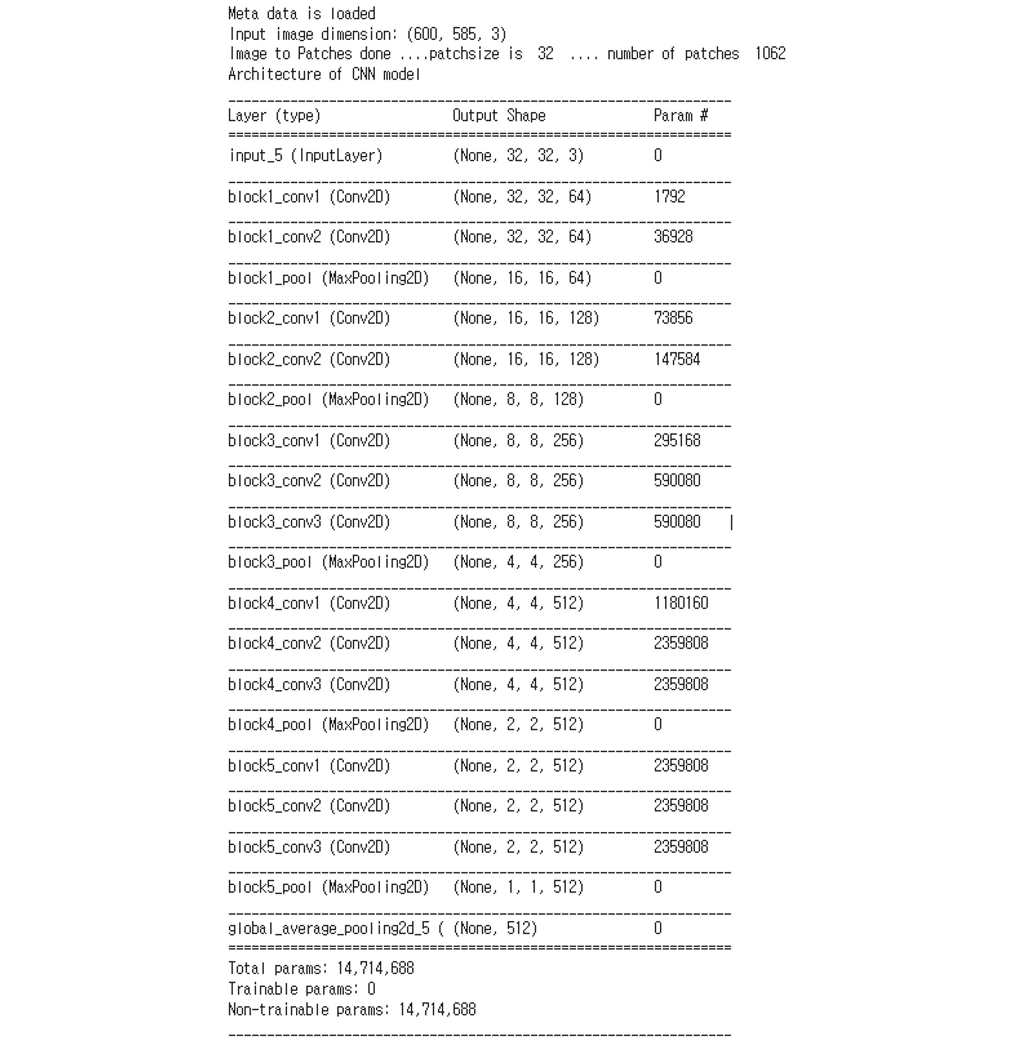
block1_conv1의 파라미터 개수는 1792임을 알 수 있는데, 이는 다음과 같이 구할 수 있습니다: 1792 = 64 × (32 × 3 + 1), s.t. K = 64, F = 3, C = 3. 또한, block2_conv2의 파라미터 개수는 147,584개임을 알 수 있는데, 이는 다음과 같이 구할 수 있습니다: 147,584 = 128 × (32 × 128 + 1), s.t. K = 128, F = 3, C = 128. 개인적으로 TensorFlow를 통해 빌드업을 했을 때 다음과 같은 구조이거나 그와 유사한 구조일 것으로 추정하고 있습니다.
# 다음과 유사한 형태일 것이라 추정

model = tf.keras.Sequential([
  # VGG16 CNN Architecture을 참고
  layers.Input(shape = (64,64,3)),
  layers.Conv2D(filters = 64, kernel_size = 3, padding='same', activation='relu'),
  layers.Conv2D(filters = 64, kernel_size = 3, padding='same', activation='relu'),
  layers.MaxPooling2D((2,2), strides = 2),
  layers.BatchNormalization(),
  layers.Conv2D(filters = 128, kernel_size = 3, padding='same', activation='relu'),
  layers.Conv2D(filters = 128, kernel_size = 3, padding='same', activation='relu'),
  layers.MaxPooling2D((2,2), strides = 2),
  layers.BatchNormalization(),
  layers.Conv2D(filters = 256, kernel_size = 3, padding='same', activation='relu'),
  layers.Conv2D(filters = 256, kernel_size = 3, padding='same', activation='relu'),
  layers.Conv2D(filters = 256, kernel_size = 3, padding='same', activation='relu'),
  layers.MaxPooling2D((2,2), strides = 2),
  layers.BatchNormalization(),
  layers.Conv2D(filters = 512, kernel_size = 3, padding='same', activation='relu'),
  layers.Conv2D(filters = 512, kernel_size = 3, padding='same', activation='relu'),
  layers.Conv2D(filters = 512, kernel_size = 3, padding='same', activation='relu'),
  layers.MaxPooling2D((2,2), strides = 2),
  layers.Flatten(),
])
이상 포트래이 tech 블로그였습니다.


